HRMS Profile Data: Why Each Scan Has Its Own m/z
In an LC-MS experiment, one collects a series of MS spectra as a function of retention time. In most cases, the data matrix shares a common set of mass labels. This document covers an exception with Agilent Q-TOF data (MassHunter), where successive scans often have different mass labels. This page explains why the exception exists, how rainbow stores these data, and how to work with the results.
Some terminology
A mass spectrometer reports intensity (how much signal was seen) as a
function of m/z. One spectrum is a scan; a run is a sequence of scans
indexed by i. (You can think of i as retention time.) Within a scan,
intensity is recorded at k points, indexed by j (from 0 to k - 1);
k is the same in every scan.
Most MS instruments have unit resolution (i.e., 1 Da) and use quadrupoles to
select one m/z to pass through at a time. Since the same m/z values are selected
on every scan, the array labels (ylabels) are the same throughout. In this
document, we will call this per-array labeling.
In Q-TOF instruments, each ion is accelerated through the same voltage to give it the same amount of kinetic energy. Ions of equal charge then separate by mass: lighter ones travel faster and reach the detector sooner, heavier ones later. The instrument records intensity against the flight time each ion takes, on a ladder of times fixed by its clock, and m/z is computed from each flight time afterward. That computation is redone every scan, so each scan has its own m/z labels. We will call this per-scan labeling.
Note
This is the high-resolution data Agilent MassHunter stores in MSProfile.bin.
Centroid vs profile
High-resolution instruments like Q-TOFs create a lot of data, so it is common to offer two storage options. A profile dataset keeps all the points from each scan, whereas a centroid dataset only keeps the peaks (Fig. 1). One must consider the per-array vs. per-scan issue for both dataset formats.
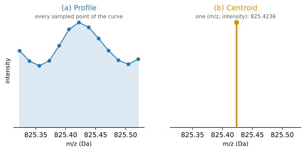
Fig. 1 One real Q-TOF peak (cyan.D, scan 0), stored two ways. (a) The profile
keeps every sampled point of the curve; (b) the centroid keeps a single
(m/z, intensity) for that same peak.
Why do mass labels change with time? Drift.
As batches of ions go through the flight tube, the instrument counts ions on an evenly spaced ladder of flight times (microseconds). These flight times are converted to m/z ratios by a process called calibration (see below). The calibration changes from scan to scan (“drift”), and thus, the m/z labels are scan-dependent (Fig. 2).
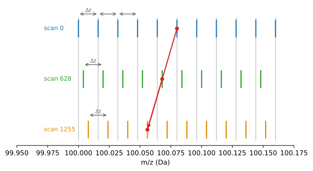
Fig. 2 Drift causes m/z labels to be scan-dependent. Because the drift is small relative to the flight time spacing, the combs do not overlap.
Calibration functions
The conversion from flight time to m/z is a calibration function, a polynomial fitted per scan. Its core is a quadratic in the flight time \(t\),
so m/z grows with the square of the flight time, with two fitted numbers
\(A\) and \(t_0\) per scan. A small polynomial correction (up to six
more coefficients \(c_n\), evaluated with numpy.polyval() on the flight
time clamped to the calibration’s valid range) is then subtracted on top so the
result reproduces the masses Agilent MassHunter reports.
Writing the whole conversion out for scan
\(i\) at flight time \(t_j = \mathrm{tof}[j]\):
The flight-time ladder \(\mathrm{tof}\) is shared by every scan; only the coefficients \(A_i, t_{0,i}, c_{n,i}\) belong to a particular scan. So rainbow never stores a full m/z value for every point of every scan, which would be enormous. It keeps the one shared \(\mathrm{tof}\) array plus each scan’s handful of coefficients and recomputes a scan’s m/z on demand: small, exact, and drift is just those coefficients changing from scan to scan.
Note
In practice, the calibration usually changes only a little between scans. However, any of the coefficients could change, so rainbow stores all of them.
The data matrix: same index, different m/z
With per-scan labels, the intensities are stored as a matrix data[i][j]:
row
iis the scancolumn
jis the point (one of thekpoints in that scan)
The matrix is rectangular, but a column does not carry a single m/z
(Fig. 3). Each column j is a fixed flight time, but the
per-scan calibration assigns it a different m/z in each scan, so data[5][j]
and data[1200][j] are intensities at different masses even though they sit
in the same column.
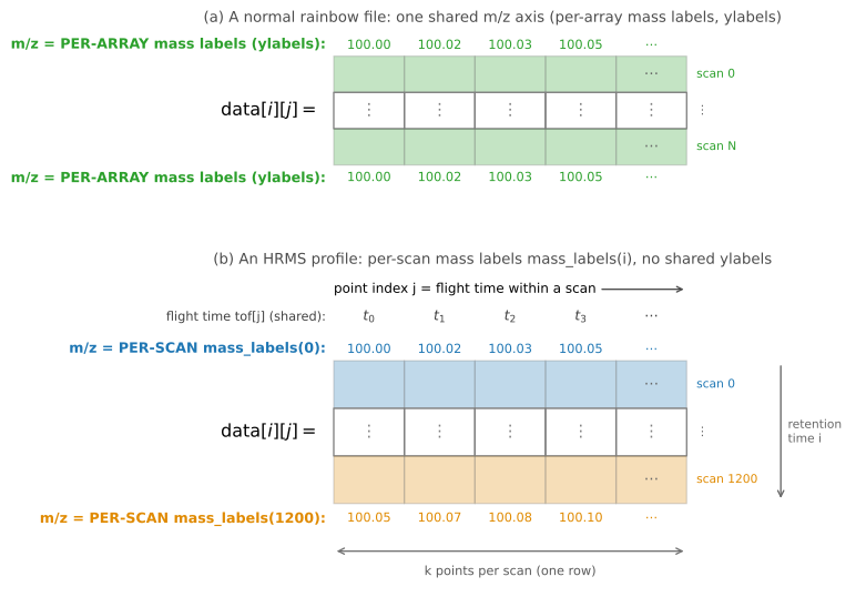
Fig. 3 (a) A normal rainbow file: each column is an m/z (per-array mass labels,
ylabels), shared by every scan (one colour, repeated above and below the
matrix). (b) An HRMS profile: columns are a shared flight time tof[j] and
the m/z is per-scan mass_labels(i) (the top strip mass_labels(0) and
bottom strip mass_labels(1200) carry different labels), so there is no
single ylabels.
Reading an HRMS file
To read a MassHunter profile dataset:
import rainbow as rb
datadir = rb.read("example.D", hrms=True, precision=4)
profile = datadir.get_file("MSProfile.bin")
This requests the per-scan representation (with precision=4 the m/z
labels are rounded to four decimals; the default precision='auto' also picks
four for Q-TOF data). To access those data:
profile.scan(i)         # -> (m/z array, intensity array) for scan i
profile.mass_labels(i)  # -> the m/z array for scan i (its own, per scan)
profile.tof             # the shared flight-time axis (same for every scan)
profile.data            # the 2-D intensities, shape (num_scans, k)
Note that there is deliberately no profile.ylabels. (If you try to access
ylabels, you will be scolded.)
If you must have one m/z axis
Per-array mass labels are convenient: one m/z axis you can index, slice, and stack. Per-scan mass labels are faithful: every point on its own correct axis. What if you want both: one shared axis you can index, that still covers every point the per-scan form keeps?
The answer is the common grid: pass a bin_width to rb.read:
import rainbow as rb
datadir = rb.read("example.D", hrms=True, precision=4, bin_width=0.01)
profile = datadir.get_file("MSProfile.bin")   # a shared-grid DataFile
profile.ylabels                               # one m/z axis you can index
Binning is performed as follows:
lay down a grid of evenly spaced bins, each
bin_widthwide, across the m/z rangedrop each scan’s intensity into the bin its m/z falls in
throw away every bin that stayed empty in all scans (Fig. 4)
The surviving bins become the columns: the union of the bins the scans occupied.
(In rainbow this is implemented by the bin_to_grid function in
rainbow/agilent/masshunter.py.)
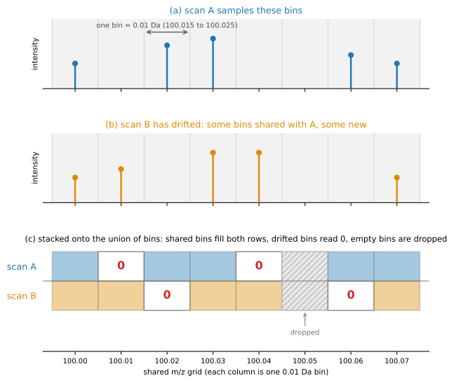
Fig. 4 Building the common grid. (a) Scan A drops its intensities into 0.01 Da bins. (b) Scan B has drifted, filling some of A’s bins and some new ones. (c) Stacked onto the union: a shared bin fills both rows; a drifted bin reads 0 (red) for the scan that missed it; and a bin empty in every scan (100.05 here) is dropped, so it never becomes a column. Shaded boxes represent non-zero intensities.
Note that there are no all-zero columns. If there is no intensity in a given bin
for any scan, it is dropped. However, there can be many sparse columns. We can see this
effect in cyan.D.
At a fine bin_width of 0.0001 Da, the scans almost never land in the same bin,
so every one of the ~315,000 columns holds exactly one nonzero entry and two thirds
of every row is zero. Coarsening bin_width pools the drifting scans, trading
resolution for fewer zeros. Once a bin is wider than the drift it catches all the scans
at once, and the zeros vanish (Fig. 5).
|
columns |
zeros (per row) |
|---|---|---|
0.0001 Da |
~315,000 |
67% |
0.001 Da |
~297,000 |
65% |
0.01 Da |
~147,000 |
29% |
0.05 Da |
~48,000 |
0% |
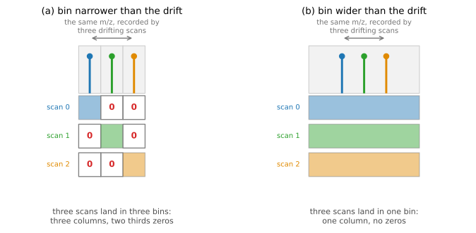
Fig. 5 Effectiveness of the common grid. (a) A bin narrower than the drift puts the three in separate bins: three columns, two thirds zeros. (b) A bin wider than the drift catches all three in one bin: one column, no zeros.
Note
bin_width is unrelated to precision. bin_width controls how
aggressively scans are pooled onto the common grid; precision only controls
how the m/z labels are rounded. If precision is too coarse to give every
bin a distinct label, rainbow warns but still bins at the requested
bin_width.
Centroids
Since centroid data are merely generated from profile data, both formats are subject to drift, and both bin the same way, producing the same zeros. The only difference is how many points sit under a peak: a profile spends many (a wide row of staircases, Fig. 6 a), a centroid spends one (a single staircase, Fig. 6 b). Both are about two-thirds zeros, but the centroid’s matrix is far smaller, so binning it is cheap.
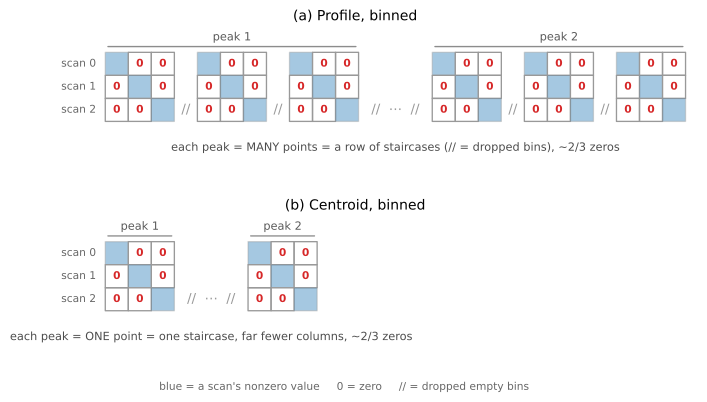
Fig. 6 The same two peaks, binned on a fine grid. Every measured point becomes a
3-column staircase, one bin per scan, and empty bins between are dropped
(//). (a) A profile spends many points on each peak, so each peak is a wide
row of staircases. (b) A centroid spends one point per peak, so each peak is a
single staircase, far fewer columns. Both are about two-thirds zeros.
A worked example
We can now put the pieces together on a real run. amber.D is a 500-scan
Q-TOF acquisition, windowed to the m/z region around 825.42 to keep the fixture
small. Read it per-scan (the default), then bin onto a shared grid, once finely
and once coarsely, and view each as a heatmap:
import numpy as np
import matplotlib.pyplot as plt
from matplotlib.colors import LogNorm
import rainbow as rb

# Per-scan (the default): each of the 500 scans keeps its own m/z axis.
profile = rb.read("tests/inputs/amber.D", hrms=True).get_file("MSProfile.bin")

# Pass a bin_width to project onto one shared grid (a DataFile with ylabels).
fine = rb.read("tests/inputs/amber.D", hrms=True,
               bin_width=0.005).get_file("MSProfile.bin")
coarse = rb.read("tests/inputs/amber.D", hrms=True,
                 bin_width=0.05).get_file("MSProfile.bin")

# fine.data / coarse.data are (num_scans, num_bins): plot either as a heatmap.
grid = fine                                     # or coarse
cmap = plt.get_cmap("viridis").copy()
cmap.set_bad("0.85")                            # render the masked zeros as grey
plt.imshow(np.ma.masked_equal(grid.data, 0),    # mask zeros so the gaps show
           aspect="auto", cmap=cmap, norm=LogNorm(),
           extent=[grid.ylabels[0], grid.ylabels[-1], grid.data.shape[0], 0])
plt.xlabel("m/z (Da)"); plt.ylabel("scan (retention time)")
plt.colorbar(label="intensity"); plt.show()
Fig. 7 shows both grids. On the fine grid each scan samples a comb of m/z positions, so most cells are 0 (grey): the zeros from binning, drifting slowly down the run. On a grid wider than the drift the comb closes up and the scans realign. The bright horizontal band is the analyte eluting off the column at one retention time. Centroids bin the same way but are far sparser (Fig. 6).
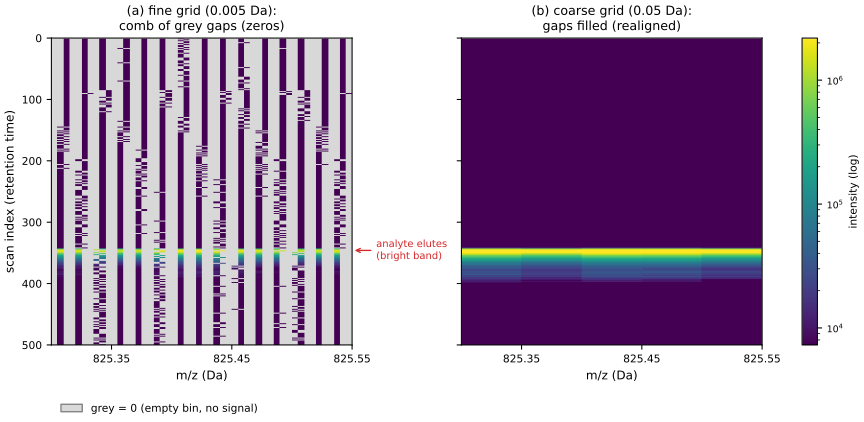
Fig. 7 amber.D (a 500-scan Q-TOF run) binned near m/z 825.42, as heatmaps: rows
are scans (retention time), columns are m/z, log colour is intensity, and
grey is 0. (a) A fine grid (0.005 Da) leaves a comb of grey gaps, the
zeros. (b) A grid wider than the drift (0.05 Da) fills them in (realigned). The
bright band is the analyte eluting.